October 23,2022

Ch-1: Reliable, Scalable and maintainable applications

• reliability, The system should continue to work correctly even in the face of adversity (hw, sw or human).

  • faults (either synthetic or natural) are when only part of the system misbehaves, If the whole system goes down then it is a failure.
  • Fault tolerance machinery can be tested and kept upto date by voluntarily turning of part of the system to see how the system fares in times of faults.
  • Hardware Faults (HDD crash, Faulty RAM, blackout, etc)
    • HDDs have a Mean Time To Failure (MTTF) of about 10 to 50 years => on a cluster of 10,000 disks, one disk might die per day.
    • This can be overcome with have a RAID setup, dual power supplies and hot swappable CPUs
  • Software Errors Weakly correlated failures across systems.
    • Software bug in linux kernel on June 30, 2012 due to a leap second
    • Runaway processes using up CPU, memory and disk
    • These bugs could lie dormant for a long time without any issues and have the potential to bring the whole system down.
  • Human Errors Any system designed to be used/operated by humans should have a high degree of flexibility because humans are known to be unreliable
    • well-designed abstractions, APIs, and admin interfaces making it easier to access “the right way” and discouuraging the wrong way
    • Sandbox environments for people to play with
    • Test thoroughly at all levels, from unit tests, integrations tests and manual tests.
    • Quick and easy recovery in case of a failure

• Scalability, As the system grows (data volume, traffic volume or complexity), system should be able to handle it.

  • What is load ? Load can be described in many ways. the load parameters are dependent on the architecture of the system. it can be, requests per second, read write ratio in the DB, sinultaneously active members in a chat room, or something else.
    • eg. Twitter, broadly has two ops post tweet user can publish a new message to their followers (12k req/s at peak), Home timeline A user can view tweets posted by the people they follow.
      • 12K req/s is easy to handle. But, the problem comes due to fan-out, where each user follows many people and each one of them follow a lot more.
      • There are broadly two approaches
        1. When a user requests their home timeline, look up all the people they follow, find all the tweets for each of those user and merge them by time.
        2. Maintain a cache for each user’s home timeline, like a mailbox of tweets for each recipient. When a user tweets, lookup all their followers and insert it in their timelines. While this approach offloads a lot of computing ahead of time. Some times there might be requirements where a lot of users have a lot of followers in those cases the computation is just very high.
        3. In a hybrid approach twitter now marks users with significant followers and uses (1) for them and (2) for others
  • What is performance?_ Once we’ve described the load, we can investigate what happens when the load increases. in online services it is responce time, in data processors it is throughput
    • Even if we make the same request over and over again, we’ll get slightly different response time on every try. And this can vary wildly due to various reasons. Hence It is better to represent this as a distribution .
    • Average time of a service is generally taken to mean the arithmetic mean but, it is not really a good measure.
    • Percentile is a better measure for response times, p50 of 200ms is the measure of the median which means that, This is a probability function, which means that atleast 50% of a request would have less than 200ms response time.
      • The outliers can be measured by p95, p99, p999 and so on. These are called tail latencies , if p95 is 10s then it means that 95 % of all requests take less than 10s. tail latencies are important for critical services like aws and others.
    • These percentiles are often used in Service Level objectives (SLOs) and service level agreements (SLAs), contracts that define the expected performance and availability of a service.
    • High percentiles become important in services which are valled multiple times as part of serving a single end-user request. The final request can b only as fast as the slowest request
    • Approaches for comping with load , Architectures are different for one load vs 10X the load.
      • REsources can be scaled up or scaled out. Distributing load across multiple machines is called Shared nothing Architectures, services can also be elastic meaning being flexible to load and scale up/out based on load.
      • Generally Stateful services are hard to scale than stateless services. This means, the database is kept as a monolith than distributing it.

• Maintainablility, System should be robust to change and be productively extensible

  • operability Make it easy for operations teams to keep the system running smoothly.
    • Monitoring, tracking down problems, keeping the platform up to date, Keeping tabs on system as a whole
    • Defining processes that make operations predictable and help keep the production environment stable.
  • Simplicity, Complexity in software slows everyone down and brings down productivity, these are complex systems are called a big ball of mud . Software which is easier to understand.
    • there are several possible symptoms of complexity __explosion of the state space, tight coupling of modules, tangled dependencies, inconsistent naming and terminology, hacks to solve performance problems, special-casing to work around issues elsewhere

Ch-2 Data models and Query Languages

Data models impacts How we think about the problem making it an important part of decision making.

The idea behind an API is that it, hides the complexity of the layer below it

Data models can hide a lot of complexities on what they do and don’t allow. This makes it important to decide the underlying data model used.

• Relational Model Vs Document Model

  • in 1970, relational model was a theoretical proposal, mid 1980’s RDBMSes have become the tool of choice for people.
  • before relational model, developers had to think a lot about the internal representation fo the data in the database. The goal of the relational model was to hide that implementation detail behind a cleaner interface
  • Other models like, Network model and hierarchical model were the main alternatives, but the relational model came to dominate them.

• Birth of NoSQL is a new attempt to overthrow SQL. A few factors for the adoption of NoSQL databases

  • A need for more scalability, which is hard for relational data, while trivial to do with Non-relational databases
  • Specialised query operations that are not well-supported by the relational model
  • Frustration with the restrictiveness of relational schemas and a desire for a more dynamic and expressive data model.

• Object-relational Mismatch Most languages are Object Oriented, This means there is an awkward translation layer is required between the obects in the application code and the database models and sometimes application models and database models drift away, this is called impedence mismatch

ORM frameworks can reduce the amount of boilerplate required for this translation.

eg, a resume in linkedin can be represented like, so

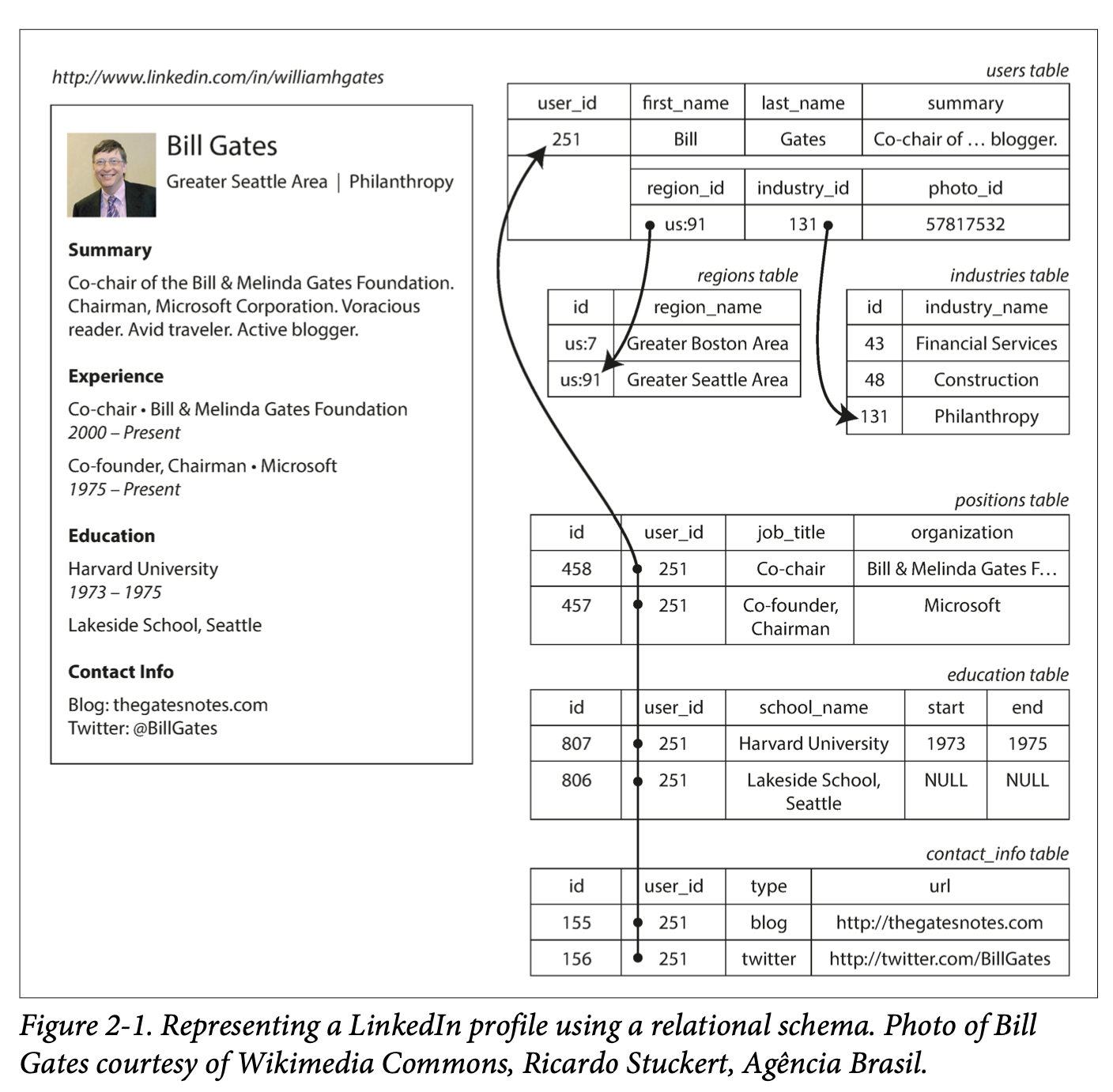(example given in “Designing Data intensive applciations”)

For sucha document, JSON has the appeal of being much simpler than XML. Document-oriented databases like MongoDB. For example the same document can be represented like, so.

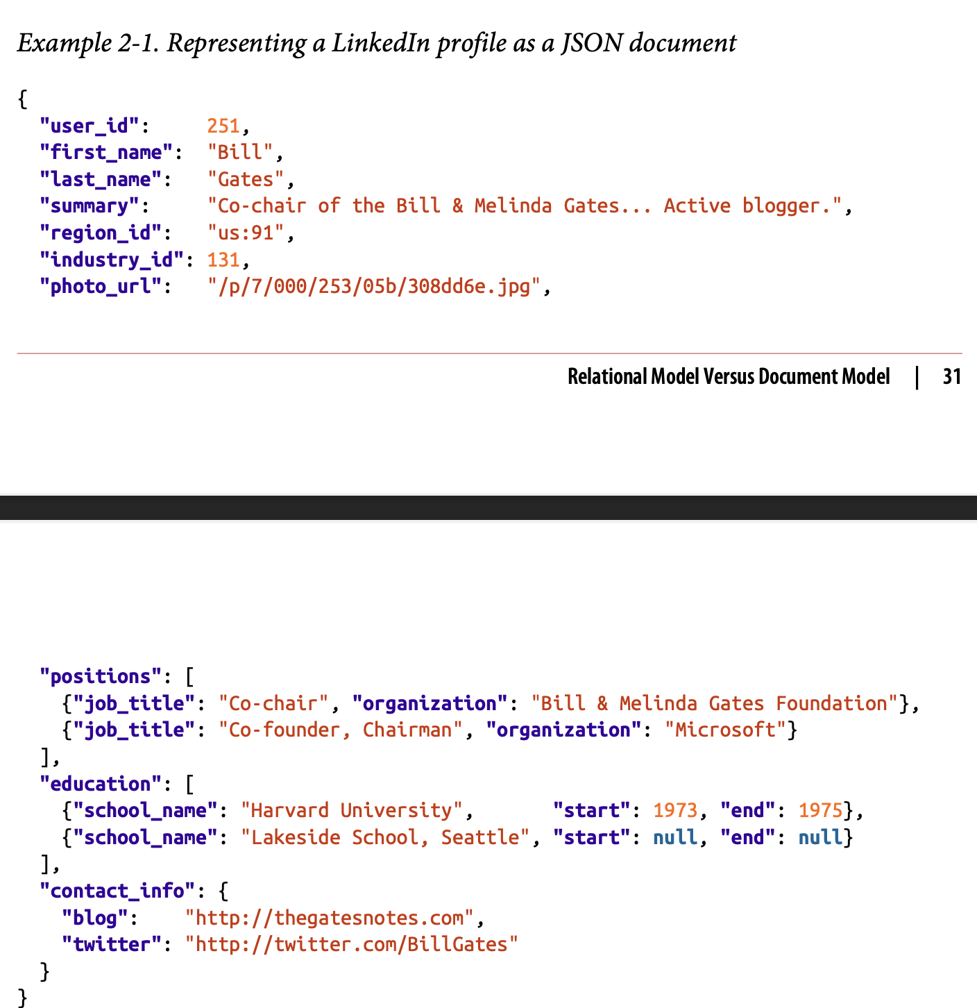(example given in “Designing Data intensive applciations”)

JSON’s unstructured format can be an issue in some use cases. But, it provides better locality. The one to many relationships from user’s positions educational history and contact info imply a tree structure.

Many-to-one and Many-to-Many Relationships

If the user has free-text fields for entering the region and the industry, then it makes sense to store them as plain-text strings. But, having a dropdown list with pre-assigned values has it’s own benefits

• Consistent style/spellings
• Remove ambiguity
• Ease of updating
• Localization support - easier while translating
• Better search

Generally Human understandable/used words can change, So it is better to use references, and use ID for the word everywhere else. Because Human known words can and do change (name of a city, person, place or thing for example). The rule of thumb is that we use references in places where human understandable words are used. This, reduces duplication while also giving flexibility to change in the name.

Normalising of this type of data uses a _many to one _ relationship. This does not fit nicely into the document model. In relational databases, it is normal to refer to rows in other tables by ID, because joins are easy. But, in document model joins are a lot harder perform because multiple queries will have to be performed.

In the resume example, we could simplify it by making schools as entities And then referencing them in the resume. This allows us to group people from same school together. Making people as entities would let us build features like, a section where people can recommend each other.

In some ways, NoSQL might be repeating history. IBM’s Information Management System (IMS) developed in 1968, used a model called hierarchical model , Which has similarities to JSON. IMS Worked well for one to many scenarios, it didn’t fare well with many to many scenarios. In those times to solve the limitations of the hierarchical model, two new model of data representation where bought out, Relational model and network model The network model, even though had a fan following has basically faded into obscurity.

The network model

The network model was standardised by Conference on Data System Langugages (CODASYL). This CODASYL model was implemented by several database vendors.

CODASYL model was a subset of the network model where each entity only had one parent, while the network model could have n parents. These were referenced with each others, unlike in SQL, these references were more like pointers, than IDs even though they were stored in the Disk.

This means, that every data had an access path and these path had to be traversed from the root node, like you would traverse a linked list. Even the CODASYL committee agreed that, this is like traversing an N-dimensional data space.

Relational model

Simple => a relation (table) is just a collection of tuples (rows)

• Any/all rows can be matched and read based on a column designated for keys.

in RDBs the query optimiser decides which parts of the query to execute in which order and what indexes to uses. => basically an access path query optimisers are complex entities and cool thing is that once you create a query optimiser, all applications that use it can leverage it.

Schema flexibility in document model

document models have no schema and that is a big advantage => all schema evaluation can be enforced at the application level, instead of the database level. => makes document model very flexible, while the relational model is rigid and requires big migration of the database to add/remove columns.

Data locality for queries

if data is accessed often, having all the data in the same locality is better for performance. This is how document databases operate and makes it better for performance. relational database might not guarantee that all data for a particular query would be in the same segment in memory and might require multiple seeks to complete.

Google spanner database offers same locality properties in relational data model, by schema to declare rows taht should be interleaved. Most relational databases also support XML and json formats. Postgres has a jsonb format which stores json data in an optimal format making it easier to index data inside json blobs.

Query Languages for data

SQL is a declarative query language while, IMS and CODASYL have imperative query language

Most common programming languages are imperative. Meaning, they’ll have to be clear about what they say and achieve.

function getSharks() {
  var sharks = []
  for (var i=0; i<animals.length; i++) { 
    if (animals[i].family === "Sharks") {
      sharks.push(animals[i]);
    }
  }
  return sharks; 
}

eg of imperative language

this is almost equivalent to the relational algebra,

sharks = σ_family = _“Sharks” (animals)

where, σ is the selection operator, returning only those animals that match the condition family = “Sharks”.

in SQL this would be, SELECT * FROM animals WHERE family='Sharks';

imperative => you decide the pattern of access, you decide the way to filter and everything else declarative => We dictate, how we want the data and the final conditions of the data, not how to fetch it. The data implementation detail is essentially hidden from the user and the database is allowed to make decisions based on the data it has. like, cleanup jobs and memory journaling.

Queries on the web

css queries in html documents are an example of declarative queries as well.

For example

li.selected > p {
  background-color: blue ;
}

this is a query that basically says all selected list item with paragraph should be blue

alternatively this can be done more verbosely in javascript by

var liElements = document.getElementsByTagName("li"); for (var i = 0; i < liElements.length; i++) {
  if (liElements[i].className === "selected") { var children = liElements[i].childNodes; for (var j = 0; j < children.length; j++) {
    var child = children[j];
    if (child.nodeType === Node.ELEMENT_NODE && child.tagName === "P") {
      child.setAttribute("style", "background-color: blue");
    }
  } }
}

which is a lot more verbose. and this has the disadvantage of not using the optimisations offered by the browser itself.

Map reduce

Map reduce is a model to process large amount of data across many machines.

eg, counting the number of elements in a db this can be done by querying for all observations with the criteria and then counting them. example, SELECT data_trunc('month', observation_timestamp) AS observation_month, sum(num_animals) AS total_animals FROM observations WHERE family='Sharks' GROUP BY observation_month

in map reduce can, this can be done by

db.observations.mapReduce( 
    function map() { //2. Map, called once for every document
      var year = this.observationTimestamp.getFullYear(); 
      var month = this.observationTimestamp.getMonth() + 1; 
      emit(year + "-" + month, this.numAnimals); //3 emit string of format "2014-12" and a value
    },
    function reduce(key, values) { //4. emitted values from map go here as args. This is then processed
      return Array.sum(values); 
      },
    {
      query: { family: "Sharks" }, //1.Query filter
      out: "monthlySharkReport"
    });

This enables us to perform distributed queries. But, nothing is stopping SQL DBs to not do the same. They are able to handle the same very well as well.

Graph like Data Models

Graph DBs are very useful in one-to-many cases. But, relational models can only handle simple cases of relations. In cases where much more complicated Databases are required, a graph database makes a lot more sense. Graph DBs generally have vertices and edges some examples include

• social graphs, Vertices are people and edges indicate which people know each other
• web graph, Vertices are web pages and edges indicate HTML links to other pages
• Rail networks, Vertices are junctions, and edges represent the roads or lines between them

Navigation systems, Shortest path finding algorithms can work on these databases

Property graphs

Each vertex consists of

• A unique identifier
• A set of outgoing edges
• A set of incoming edges
• A collection of properties(kv pairs)

Each edge consists of

• A unique identifier
• The vertex at which the edge starts (the tail vertex)
• The vertex at which the edge ends (the head vertex)
• A label to describe the kind of relationship between the two vertices
• A collection of properties (key-value pairs)

In this model, both vertex and edge can be tables in a DB and everything can be done using queries for example, A property graph can be created using

Triple-Stores and SPARQL

The triple-store model is mostly equivalent to the property graph model. in a triple-store, all informations is stored in the form of very simple three-part statements: (subject, predicate, object). for example,

(Jim, likes, bananas). The subject is equivalent to a vertex in a graph.

Cypher Query language

query language for property graphs

Ch-3 Storage and retrieval

• simplest database possible.
  • append data to a file in comma seperated fashion. fetch when required eg,

    db_set () {
    echo "$1,$2" >> database
    }
    db_get () {
    grep "^$1," database | sed -e "s/^$1,//" | tail -n 1
    }
  

  • writes are fast, read is slow as O(n).
  • To effectively find the keys we need an index . But writing to the index takes extra time during writes, slowing it down
  • The tradeoff is, wellchosen indexes fasten queries. But, slowdown writes
  • Simplest index would be a hashmap which stores the offset of the data in the file. making it faster to fetch Usecase, we need to record number of times a video is played.
  • We can only append to a file. break the file into even sized chunks, when it reaches a certain size. compaction can then be performed on these segments.
  • While compaction is happening, reads can still happen in the old files. Merging of multiple segments can also be done, without impact to reads
  • Here, every segment has its own hashmap. To find a key, we check in the recent segment’s hashmap and then the next and then the next.
  • file format binary blob is better than csv
  • Deleting When deleting a special record is made against that key. While merging, those keys are deleted
  • Crash recovery Hashmap creation for every segment while startup would be slow. writing down index to disk helps in that
  • Partially written records When database crashes while appending, it could mangle the data. Bitcask files include checksums, allowing corruption detection
  • Concurrency control have only one writer thread. Reads, can be concurrent
  • This only works if the hashtables fit into memory. Hash maps on disk is finnicky. Range queries are not efficient

SSTables and LSM-Trees

• In the same above structure, we can store logs in string sorted format . Also, a key only appears once in a merged segment

• maintain a memtable before writing anything down. when the memtable becomes bigger than a threshold. Write to disk as an SSTable file.

• While reading, we can try the memtable first and in the most recent disk segment and the next and so on.

• Occassionally Merge segments with these properties => compaction + merge

SSTables, idea works very well because, the idea of adding log files sequentially increases throughput. While, compaction running in the background, enables fast fetch from the disk I/O.

B-Trees

introduced in 1970 and “ubiquitous” within 10 years.

• Keys are stored in sorted key-value pairs.
• in log-structured indexes writes are done by appending to file of specific segment. But, in B-trees data is written in fixed sized blocks called blocks or pages, generally 4KB.
• Each page can be identified using an address or location. Pages can refer each other. Sort of like pointers, but for hard disk.
• One page is called the root of the b-tree. All lookups start here.

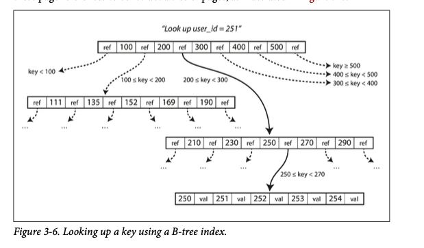(example given in “Designing Data intensive applciations”)

• The keys are branched out based on ranges. in the above example fi we are trying to find 252 key. Then in the root node we can predict that we will have to look at the ref in between 200 and 300. and in the next level between 250 and 270.
• For updates, we want to update the value of an existing key in a B-tree. then we search for the leaf node and then insert the data. if the page is full, then we split the leaf node and update the parent. like so,

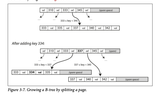(example given in “Designing Data intensive applciations”)

The algorithm ensure that the tree remains balanced: a B-tree with n keys always has a depth of O(log n). Data can be fit in 3 - 4 levels. So not a lot of page references are required. 4KB page with branching factor of 500 at 4 levels can store upto 256 TB

B-tree reliability

• New data in a page is written by overwriting a page on disk with new data. The working assumption is that the reference does not change.
• Overwriting a page on disk is a hardware operation and can limit the actual write throughput. in SSDs
• A write ahead log (WAL) is used to recover from database crashes. This is an append-only log of the operation about to be performed.

B-tree Optimizations

• LMDB uses copy-on-write instead of overwriting. copy on write, copies the file to a new location and edits the file and updates the reference in the parent
• page space can be saved by storing abbreviated keys. more keys per page => bigger branching factor => greater performance
• Since the pages can be across the disk. Disk seeks becomes expensive this can be overcome by writing sequentially. It is difficult to maintain that order as the tree grows, which is where, LSM trees perform great.

LSM vs B-Tree

• By nature of the algorithms LSM-trees are faster than B-trees for writes. While B-trees are faster for reads. This is Because LSM-trees would have to check multiple structures to find a key. While B-trees are consistently O(log n)

LSM-tree advantages

• B-tree => 2 writes per data => 1) WAL 2) actual data. There is also the overhead of overwriting a whole page even for small mutations.
• LSM indexes also rewrite data multiple times for merging and compaction. This act of writing multiple times to the drive for one entry in the DB is called write-amplification
• In write-heavy applications, the performance bottleneck will be the write throughput. LSM-trees are able to sustain higher throughput because of low write-amplification.
• Also, sequential writes makes writing to disk much faster
• LSM-trees can be compressed better => information density is high.
• B-trees have wasted space due to fragmentation.

LSM-tree disadvantages

• Compaction can sometimes interfere with the performance of ongoing reads and writes despite, making sure compaction is incremental and without affecting concurrent access.
• At high throughputs disk’s write bandwidth needs to be shared between, initial write and compaction. This is important because, without the right balance data would be written forever, without compaction until the disk runs out of space.

Other indexing structures

• All of the above discussions assume one Primary key for indexing purposes. There can also be secondary indexes.
• A secondary index => need not have unique keys. There can be multiple values behind the same key. These are very useful in aggregate type queries.

Storing values within the index

• The key in an index is what queries search for. The value could either be the row itself or, it could be a reference to the row stored elsewhhere. In the latter case, the place where rows are stored is known as a heap file.
• heap file stores data in no particular order. When just updating files, heaps can be very effiient.
• In a lot of cases, it would be simply be easier to store data next to the index. This is called a clustered index
• Middle ground between clustered index and non-clustered index is, covering index or index with included columns, which stores come of a tables columns within the index. This could increase read speed while reducing writes.

Multi-column indexes:

• most common type => concatenated index simply combines several fields into one key by appending one column to another.
• This can be used as a more general way of querying several columns at once. eg. Geospatial data

SELECT * FROM restaurants WHERE latitude > 51.4946 AND latitude < 51.5079 AND longitude > -0.1162 AND longitude < -0.1004;

A standard BSM-tree or LSM-tree is unable to answer this query. This can be done more efficiently with multi-column indexes.

This also could be useful in cases where, we have

Full-text search and fuzzy indexes

• full text search engines allow synonyms and typos of a certain distance.
• Full text can be stored in memory in a trie like automaton. This automaton can be transformed into a Levenshtein automaton which supports efficient search for words within a given edit distance.
• in Lucene the keys are stored in a trie and then this is transformed into a levenshtein automaton

In-memory everything

• Hard-disks come packed with limitations and we tolerate this, because they are cheap + durable.
• There are another class of databases using RAM for everything.
• Durability can be achieved by writing everything in a log.
• VoltDB, MemSQL and others provide strong durability by writing to the log and writing.
• Redis and Couchbase provide weak durability by writing the log asynchronously
• The speed is not purely because all data is, in-memory Because, given enough memory in a machine, the OS loads most of the recent in memory instead of in the hard disk.
• The speed is because in-memory databases don’t have to encode data from memory to disk.
• Another benefit, is that, in-memory databases provide access to non-harddisk friendly datastructure. eg. Redis gives access to priority queues and sets.
• In some cases, in-memory databases can dump Least Recently used data to disk. This is the reverse of what the OS does with virtual memory and disk swap.

OLTP and OLAP

In Early days when computers were mostly business devices. Commercial Transactions had to be recorded. But, over time the same idea of “transaction” in databases stuck and we started using the same idea. These types of data processing is called Online transaction processing (OLTP). This has nothing to do with ACID. this just means that, the changes are instantaneous and not in batch processes

Databases are increasingly used in Data analytics as well. So, Databases started supporting data analytics changes. these data are often written by business analysts. This is called Online Analytic Processing (OLAP).

Data Warehousing

• Data present in OLTP databases can be ported to a different place where queries can be run to get results. This is called a Data Warehouse.
• Data warehouses can also be optimised for analytic access patterns.

OLTP and data warehouse divergence

• Acceess patterns are different which means that, there are increasingly different products that satisfy both needs.
• Teradata, Vertica, ParAccel are under commercial entereprise license. and only support Analytic workload. There are other open source projects like, Apache Hive, Spark SQL, Cloudera, Impala, Facebook Presto, Apache Tajo

Schemas for analytics: Stars and Snowflakes

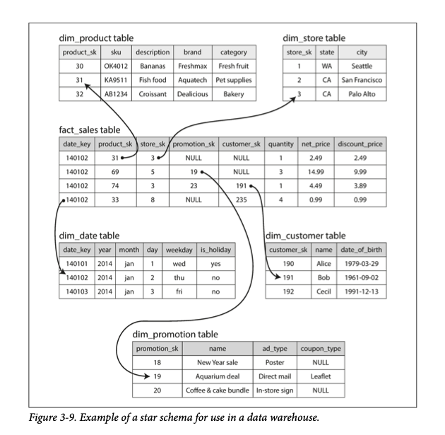
• In OLAP databases there are fact tables which holds a single event. This is used to point to other events that happened. like below.

(example given in “Designing Data intensive applciations”)

facts are usually captured as individual events, as they arrive. In the above example some are attributes, while others are references. The star name is because of the way how, fact table is in the center while dimension tables are on the outside

There is another pattern called snowflake. where the dimension tables are further broken down into other processes.

Column-Oriented Storage

• fact tables have the potential to grow to trillions of rows and petabytes of data.
• Generally, even though fact-tables can have 100s of columns. 4 - 5 are accessed per query.
• In OLTPs, data is stored in row fashion.
• in columnar storage, each column is seperated into different files and to fetch data of nth element, only the columns that are required can be loaded into memory and nth element from each file can be gotten. This reduces the search space substantially.

Column Compression

Since columnar data are one-dimensional, they can be compressed quite a bit using methods such as, run-length encoding There are different compression schema for different data types

Sort order in Column Storage:

In columnar storages. It is better to store columns in a sorted order. All columns cannot be sorted independently though, the power of the column storage comes because we know all Kth element in the columnar files represent the same row. If date_key is the first sort key, it might make sense for product_sk to be the second sort key.

Several different sort orders

A clever extension of this idea is to sort every column in several different ways and replicate them across machines. This is similar to having multiple indexes across different files.

Writing to Column-Oriented Storage

The base assumption for column-oriented storage is that, there are a lot more reads and pretty much no overwrites or in-place changes. This means that data can be easily appended to column files but not necessarily changed easily. Changing data, would take a lot of writes and would be very costly.

Aggregation: Data Cubes and Materialized Views:

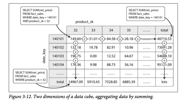
Data warehouses often perform operations like, COUNT, SUM, AVG, MIN, or MAX over a Materialised aggregate. This is usually run over a Materialised view. In a relational data model, It is like a standard/virtual view but it is written to disk. When the underlying data changes the materialised view also changes. This means increased writes and this is why it is not used in OLTP databases

In OLAP warehouses there is a common special view known as OLAP cube. It is a grid of aggregates grouped by different dimensions.

(example given in “Designing Data intensive applciations”)

In the above example, each data is represented in different ways and can be easily derived.

Ch-4 Encoding and Evolution:

Applications and their underlying data representations change over time. Application design should ideally allow flexibilty towards changes.

• In memory structures
  • objects, structs, lists, arrays, hash-tables, trees…. These are efficient to be used as in-memory structures
• To persist these data in a file/ send over a network. These in-memory structures should be made as a self-contained sequence of bytes like JSON

Problems with encoding/decoding:

• if language specific encoding is used. Cross language decoding is difficult. This inability to interoperate makes it harder to adopt and use multiple programming languages
• To restore same object/struct types the decoder needs to be able to instantiate new objects. If an attacker could make the decoder, read an arbitrary stream of bytes they will be able to make the decoder create arbitrary objects and get access to the application
• data versioning is hard.
• Very inefficient in a lot of cases

JSON, XML and CSV are popular formats and each come with their own caveat

• JSON => no int vs float distinction.
• JSON,XML => handles unicode well, but no arbitrary binary representation
• CSV => No schema, and a lot of vaguery in definition.

Binary encodings

When used, within an organization, there is scope to make the format a lot tighter than the lowest common denominator. We can customise these binary representations, based on use case

Thrift and Protocol Buffers

These are binary encoding libraries that are able to make space efficient binary representations. Thrift has to levels, Binary Protocol and Compact Protocol. in compact protocol, there are no field names only representations to them (similar to protobuf field tags that is used).

Apache Avro

Avro has writer’s schema and reader’s schema. Both schemas generate some code.

• When the bytes are being decoded both writer and reader schemas are evaluated side by side. the order of the representations does not matter
• If the writer has a field and the reader does not have the field, then that field is ignored.
• if the reader has a field and the writer does not have the field, then a default value is given.

Data Flow

Data flow through databases

Service writes, data to db and then another service reads from the database. There can be legacy data and hence migration might be required for the new application code to be able to view the data.

Data flow through Services: REST and RPC

REST uses json, mostly and is used in RPCs are used to call a function in a remote networks service.

Problems with RPCs

• Local function call is predictable to succeed or fail. Network requests are not, request/response can be lost in a network problem, machine might be slow hanging up the whole program.
• local functions return with 3 states, throw exception, return a result, or never returns. in RPCs there’s another possibility that there is a timeout
• somtimes, only responses could be dropped. in those cases we generally retry, but there is no way to know, if any of the requests got through or not.
• Network latencies are larger than local function calls
• In local function calls pointers can be passed around. But for RPCs the whole data needs to be passed around.
• RPC is language independent, so data needs to be translated into its local representation irrespective of the source language.

Data flow through Message-passing:

This is a mix of both data flow through databases and REST/RPCs. Data is sent to a database like structure from where data is then processed by services asynchronously. This includes services like, Kafka celery and others

Distributed actor frameworks

• In actor model, instead of dealing directly with threads and their problems (race conditions, locking, deadlock…), this logic is encapsulated in actors. Each actor represents a client/entity.
• Communication between actors is done through asynchronous messaging.
• Since each actor only processes one message at a time, it does not need ot worry about threads and can be scheduled independently. Also, we expect messages to be lost and that provides us with advantages
• A distributed actor framework essentially integrates a message broker and the actor programming model into a single framework. Messages are encoded and decoded over the network.
• performing rolling updates in a distributed actor framework is hard. Forward and backward compatibility will have to be handled.

Famous distributed actor frameworks

• Akka uses Java’s built-in serialization by default, which does not provide forward or backward compatibility. However protobufs can be used to handle forward and backward compatibility
• Orleans uses a custom data format and does not support rolling upgrade deployments. To deploy a new version of your application, a new cluster has to be setup and traffic should be redirected there.
• Erlang OTP Record schema changes are hard to make.

Ch-5 Replication

Data Replication is done for many reasons,

• To keep data geographically closer to users
• To allow the system to continue despite multiple failures
• To Scale out number of machines that can serve read queries

Leaders and Followers

Each node that stores a copy of the database is called a replica. Every write needs to be processed by the replica. Else, the replica would be inconsistent with the master.

Leader-based replication

• One replica is the leader/master and when it writes some change to the database it has to send the data to all the nodes as part of replication log or change stream.
• The other replicas/followers read from the change stream and update their data replica as well.

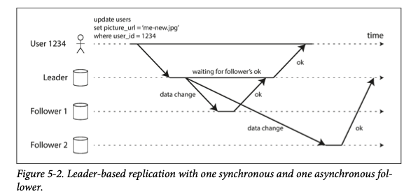
Synchronous vs Asynchronous replication

Synchronous replication is when the leader responds after all replicas are consistent with the write. Asynchronous is when The leader assumes the followers will catch up and responds to the write request after it has written to the replication log.

Asynchronous systems could lose data if the leader fails or if the message itself fails to get sent

(example given in “Designing Data intensive applciations”)

Setting up new followers.

How to setup new followers when the leader is getting updated constantly? Take snapshot of leader => copy to follower => Follower comes up and requests all change since the time of the snapshot / since the last log sequence number it has

Handling Node Outages

ability to stop/restart individual nodes is desirable => makes a robust system

• Follower Failure: Catch-up recovery, is when The follower goes down and comes back, it is able to look at the backup in its disk and request for all changes since the last request
• Leader Failure: Failover, The leader node could also go down, in those cases, we need a way to figure out who to promote to a leader
  • Determining the leader has failed, Minimum threshold for non-responsiveness. eg, if the node does not reply in 30 seconds it’s assumed dead.
  • Choosing a new leader, Controller node who elected the previous leader can be delegated the task of finding a new leader. The follower with the most upto date data could also be promoted
  • Reconfiguring nodes to follow new leader, All clients now, need to route all write requests to the leader.

Implementation of Replication Logs

There are several replication techniques

• Statement-based replication Sending the whole write query to all followers. this is harder for cases where we have to update time, random number and others as each node might compute a different value. Workarounds are possible, but generally not desired
• WAL shipping We ship the whole Write ahead log that the database is using to keep track of operations that it is performing.
• Logical (row-based) log replication This log is a very logical seperation between the database and storage. So, When an update/insert/write occurs, it is a logically isolated part, that has all the data to replicate the data.
• Trigger-based replication - We can have separate triggers based on specific change in specific areas.

Problems with Replication lag

Generally there is a time delay between data replication and the actual write. This means, depending on where the read request is landing, the data returned could be different. These challenges could be addressed differently.

• Reading Your own Writes, in a lot of cases, when the writer is asking for the write that they did, they want their most up-to-date data not stale data from a replica. This can be addressed by
  • Read from the leaer if it is the writer asking back for their write.
  • Keep track of the replication lag and read from the replica if threshold is within limits. So, that we don’t overwhelm the leader.
  • Client can remember the recent update and request for the most updated version after that.
• Monotonic Reads, This happens when the reader reads from multiple replicas that are inconsistent (for the time being).
• Consistent prefix reads, a guarantee that if a sequence of writes happen in a certain order, then anyone reading those writes will them in the same order.

multi-leader replication

Leader-based replication has the downside that if there is network interruption for the leader, then write throughput will be abyssmal. To solve cases like these, each node that processes a write must forward that data change to all the other nodes.

Multi-datacenter operation

There could be two leaders in different data centers and both leaders sync with each other and resolve conflicts and distribute that data to their followers.

• Performance, In a multi-leader configuration, every write can be processed in the local datacenter means the queries are processed faster than a single leader
• Tolerance for outages, Even when one datacenter goes down the service is up, because there are multiple leaders.

Clients with offline operation

The same idea used for multi-datacenter operation can be performed in offline operations. Basically when offline the local data store becomes the leader and when online it syncs with the leader in the datacenter.

Collaborative editing

Collaborative editing is similar to a database replication problem, when a user edits some data locally then the changes are instantly applied to their local replica and asynchronously replicated with the server. If there is to be a guarantee that there won’t be any conflicts then the writer must get a lock on the document, before they start editing. And after editing it can be delegated to someone else. This is similar to Single-leader replication with transactions on the leader.

conflicts

Synchronous versus asynchronous conflict detection, Synchronous conflict detection = single-leader replication because, you would have to wait until everyone has the data replicated.

• conflict avoidance, If the application can ensure that all writes for a particular record go through the same leader, then conflicts cannot occur. eg, same user gets the same data-center
• Converging towards consistency, Even though all replication is asynchronous we can converge to a consensus.

Technical Words:

• impedence mismatch - Drift between, ORM and actual DB model
• data normalisation - Standardising data representation by using entity reference instead of,
• Triple-Store - Model of data where, tuples of 3 are stored in graph like databases and can be queried
• Compaction - throwing away duplicate keys in the log and using only the recent ones.
• SSTables - Sorted String Tables, store strings in sorted order.
• memtable - in-memory tree
• LSM-tree - Log-Structured Merge-Tree. where data is appended in a log like fraction and merged occasionally.
• Leveled Compaction - based on LevelDB, having n-tier levels for compaction
• size-tiered compaction - Compaction done, after waiting for the file to become a certain size.
• leaf page - in B-trees leaf pages are, ones where we have come down to individual keys.
• Branching factor - maximum number of references that can be in a page in a b-tree.
• copy-on-write - A way of updating data in b-tree where the data(of a page) is copied to a new location and then the refs are updated.
• write-amplification - One write to the DB resulting in multiple disk writes.
• Clustered index - Key where data is stored near the index (e.g. InnoDB storage engine)
• covering indexes or index with included columns secondary indexes where some columns are stored within the index.
• concatenated indexes - combines several fields into one key by appending one column to another. (eg phone book which has a ’lastname-firstname’ index. it can be used to find people with certain lastname (or) people with certain ’lastname-firstname’ combination. But, totally useless if you want people with certain firstname)
• OLTP - Online Transaction Processing. A type of database operation which gurantees instantaneousness
• OLAP - Online Analytics Processing. Database operation which is not expected to be instantaneous and can be done after the fact.
• fact table - In OLAP tables, a fact table is used to represents an event that occured at a certain time.
• Run length encoding - in a one dimensional list of data, it can be reduced by counting the number of times an element gets repeated and then encoding alongside it.
• Materialized aggregate - aggregate function over a materialized view.
• Materialized view - like a standard (virtual) view, but the contents of the result is written to disk. When the underlying data changes, materilised view also changes
• OLAP cube - a materialized view with aggregate data of content
• encoding, serialization, marshalling, in-memory representation => byte sequence
• decoding, deserializaiton, unmarshalling, byte sequence => in-memory representation
• data outlives code in a lot of cases, data in the db is persisted forever while the application keeps evolving, this has implications like, backward-compatibility and database migrations.
• Service Oriented Architecture (SOA), uses discrete, self-contained services instead of monolithic architectures.
• Replica - Nodes storing a copy of the data
• leader based replication - A leader/master node streams out the write/update changes that it is receiving
• Change stream/ replication log - Change stream is the stream sent by the master node to it’s slaves.
• Catch-up recovery -
• Failover -
• Controller node -
• Logical row replication.
• Monotonic reads
• Multi-leader configuration

last update: 2024-09-06